Usage Guide
This guide provides an in-depth walkthrough of the ibbi package's functionalities. We will cover everything from installation and basic setup to advanced applications like model evaluation and explainability, complete with detailed code examples and explanations to help you integrate ibbi into your research workflow.
Installation
Getting ibbi set up on your system is a two-step process. Since ibbi relies on PyTorch for its deep learning capabilities, it's crucial to install it first to ensure compatibility with your hardware, especially if you have a GPU.
Hardware Requirements
-
Disk Space: A minimum of 10-20 GB of disk space is recommended to accommodate the Python environment, downloaded models, and cached datasets.
-
CPU & RAM: Running inference on a CPU is possible but can be slow. For model evaluation on large datasets (like the built-in test set), a significant amount of RAM (16GB, 32GB, or more) is highly recommended to avoid memory crashes.
-
GPU (Recommended): A CUDA-enabled GPU (e.g., NVIDIA T4, RTX 3060 or better) with at least 8GB of VRAM is strongly recommended for both inference and model evaluation.
1. Install PyTorch
For optimal performance, particularly with GPU acceleration, it is essential to install the correct version of PyTorch for your system (Windows/Mac/Linux) and CUDA version. Please follow the official, system-specific instructions at pytorch.org. This will ensure you leverage the full power of your hardware.
2. Install IBBI
Once PyTorch is installed, you can install ibbi from the Python Package Index (PyPI) using pip. It is highly recommended to do this within a virtual environment to avoid conflicts with other projects.
🐍 Conda Installation
# 1. Create and activate a new conda environment
conda create -n ibbi_env python=3.11 -y
conda activate ibbi_env

# 2. Install PyTorch first by following the official instructions
# for your specific system at https://pytorch.org/get-started/locally/

# 3. Install the ibbi package using pip
pip install ibbi
🟨 Pixi Installation
# 1. Initialize a pixi project in your directory (optional)
pixi init

# 2. Install PyTorch first by following the official instructions
# for your specific system at https://pytorch.org/get-started/locally/

# 3. Add ibbi to your project. Pixi will automatically handle the
# creation of the environment and resolve all dependencies, including PyTorch.
pixi add --pypi ibbi

# 4. Run commands or scripts within the managed environment
# For example, to start an interactive python session:
pixi run python
For developers who want to contribute or use the latest, unreleased features, you can install the package directly from the source on GitHub:
pip install git+https://github.com/ChristopherMarais/IBBI.git
Core Functions
The ibbi package is designed around a simple and intuitive API. The following core functions are your primary entry points for exploring, loading, and using the models.
Listing Available Models
Before you can use a model, you need to know what's available. The ibbi.list_models() function provides a comprehensive overview of all registered models, their tasks, and key performance metrics. This is the best first step to help you select the most appropriate model for your specific needs.
import ibbi

# Get the model list as a pandas DataFrame for easy viewing and filtering
models_df = ibbi.list_models(as_df=True)

# Display the full table to see all available models and their metrics
print("--- Full Model Summary ---")
print(models_df.to_string())

# You can also filter the DataFrame to find models for a specific task
print("\n--- Multi-Class Object Detection Models ---")
multi_class_models = models_df[models_df['Tasks'].str.contains("Multi-class")]
print(multi_class_models[['Model Name', 'mAP@[.5:.95]', 'F1-score (Macro)']])
Creating a Model
Once you've chosen a model, you can load it using ibbi.create_model(). The first time you load a model with pretrained=True, its weights will be downloaded from the Hugging Face Hub and stored in a local cache directory (~/.cache/ibbi by default). Subsequent calls will load the model instantly from your local machine.
For maximum convenience, ibbi provides simple aliases for the primary recommended model for each major task. This is the easiest way to get started without needing to remember specific model version names.
# Load a single-class object detection model using the "beetle_detector" alias
# This is ideal for quickly finding any beetle in an image.
detector = ibbi.create_model("beetle_detector", pretrained=True)

# Load a multi-class species detection model using its full, specific name
# This provides both location and species identification.
classifier = ibbi.create_model("yolov12x_bb_multi_class_detect_model", pretrained=True)

# Load a zero-shot detection model using the "zero_shot_detector" alias
# This model is great for general-purpose object detection using text prompts.
zs_detector = ibbi.create_model("zero_shot_detector", pretrained=True)

# Load a feature extraction model using the "feature_extractor" alias
# This is used to convert images into numerical vectors (embeddings).
feature_extractor = ibbi.create_model("feature_extractor", pretrained=True)
Prediction and Feature Extraction Examples
The models can perform inference on a variety of image sources, including a local file path, or a PIL.Image object that is already loaded in your Python script. This flexibility makes it easy to integrate ibbi into diverse data processing workflows.
NOTE: We recommend to create different instances of the model for inference and feature extraction to avoid any potential conflicts.
Example 1: Bark Beetle Detection (Single Class)
Use Case: These models are optimized to answer a simple but crucial question: "Is there a beetle in this image, and where?" They identify the location (bounding boxes) of any beetle without identifying the species. This is highly effective for initial screening of field-trap images or other raw collection data to quickly quantify the number of specimens.
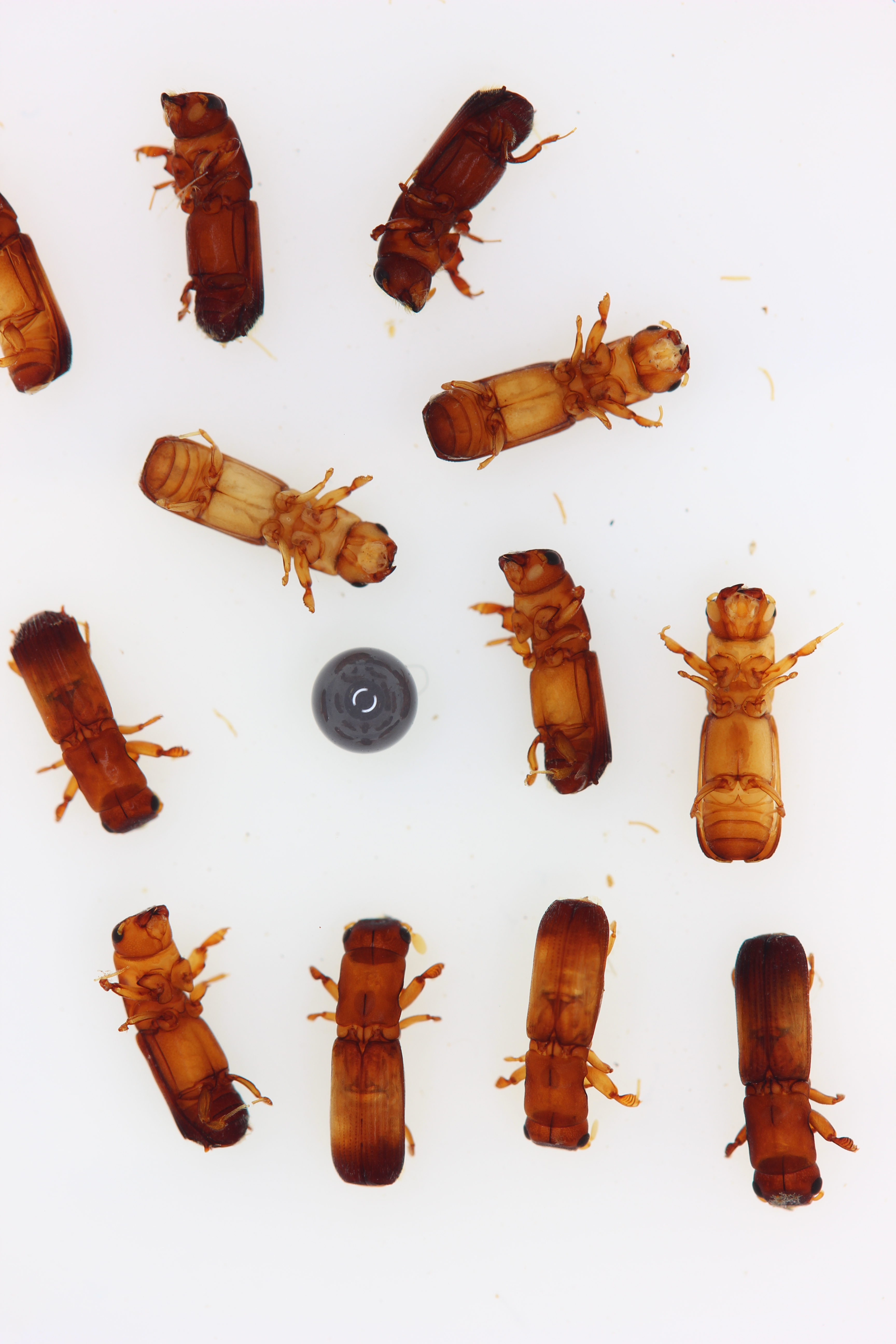
Input Image:

import ibbi

detector = ibbi.create_model("beetle_detector", pretrained=True)

# You can use a local file path
image_source = "https://media.githubusercontent.com/media/ChristopherMarais/IBBI/main/docs/assets/images/beetles.png"

# Get bounding box predictions. The model returns a dictionary.
results = detector.predict(image_source)

# The result is a dictionary containing the detected boxes, confidence scores, and labels.
print(f"Detected {len(results['boxes'])} beetles.")
# Example output for the first detected beetle:
if results['boxes']:
    print(f"  - Box: {results['boxes'][0]}")
    print(f"  - Label: {results['labels'][0]}")
    print(f"  - Score: {results['scores'][0]:.2f}")
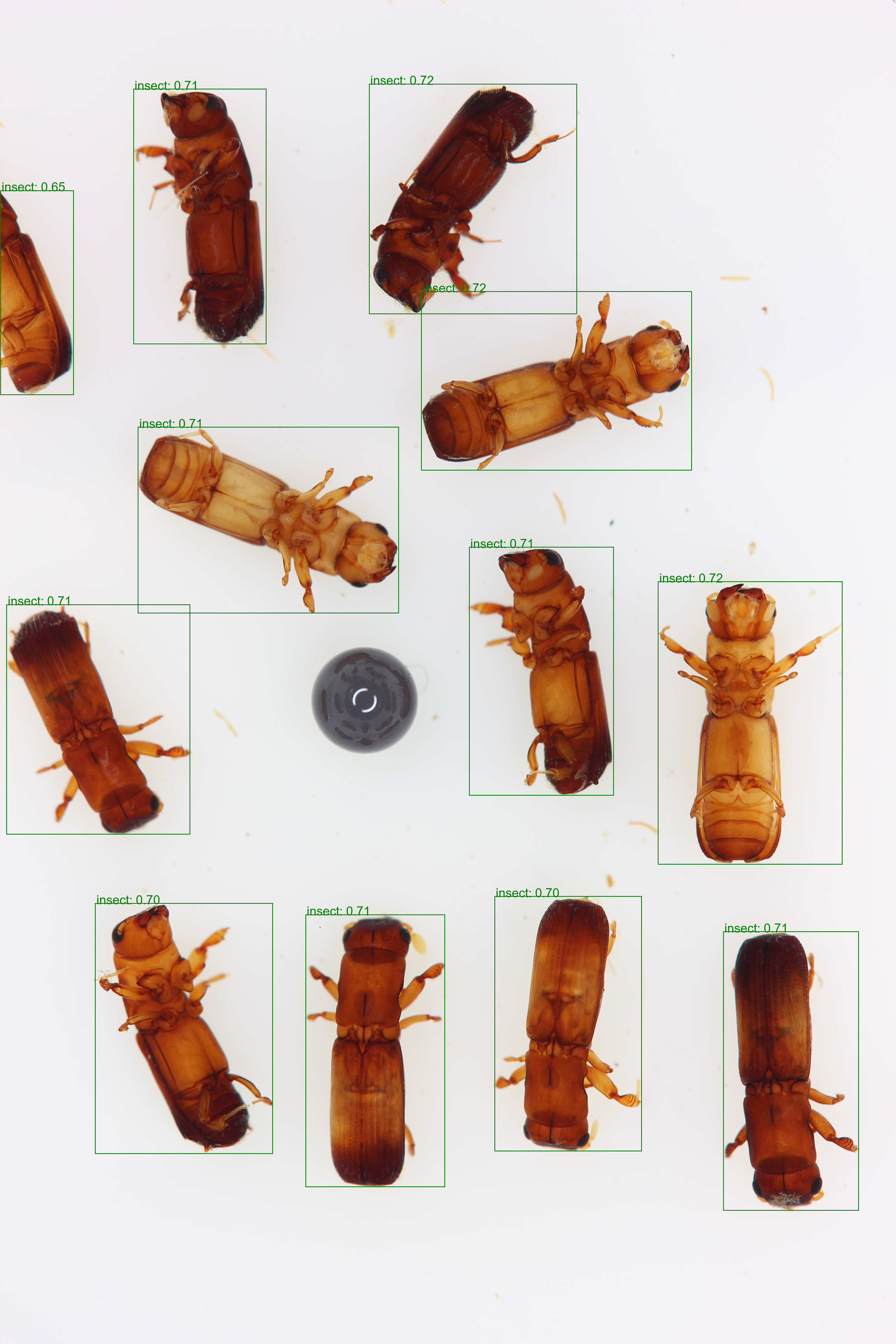
Detection Output: The output image shows the detected beetles, each enclosed in a red bounding box with its confidence score.

Example 2: Species Detection (Multi-Class)
Use Case: These models perform the core task of detailed biodiversity analysis by simultaneously finding the location of bark beetles and predicting their species. This is invaluable for species inventories, monitoring the spread of invasive species, and conducting ecological research where species-level data is paramount.
import ibbi

classifier = ibbi.create_model("species_classifier", pretrained=True)

# Use the same multi-beetle image to get species-level predictions
results = classifier.predict(image_source)

# The output is a dictionary with predicted species labels for each detected box.
print(f"Detected and classified {len(results['boxes'])} beetles.")
if results['boxes']:
    print(f"  - Top Prediction Box: {results['boxes'][0]}")
    print(f"  - Predicted Species: {results['labels'][0]}")
    print(f"  - Confidence Score: {results['scores'][0]:.2f}")
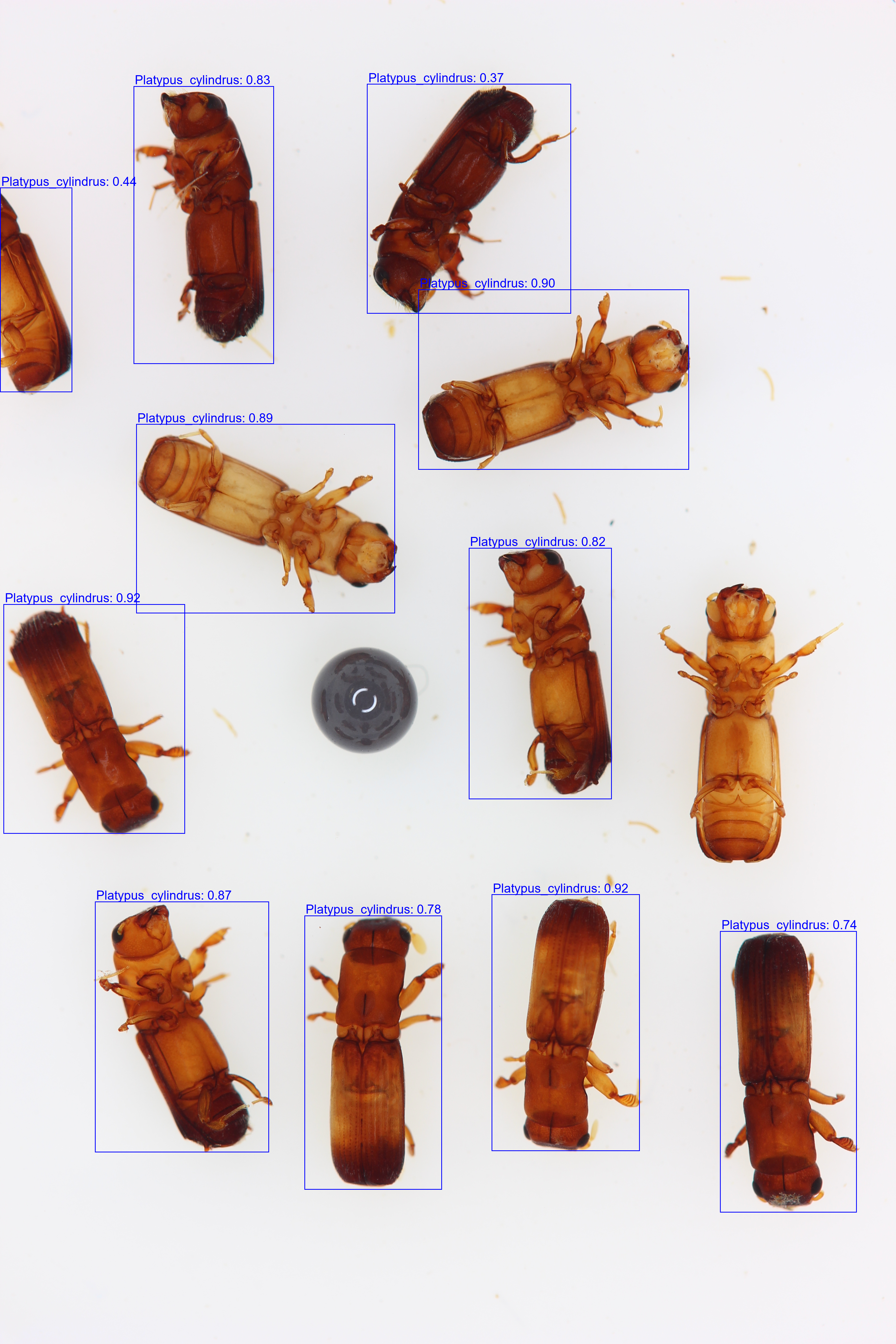
Classification Output: The output image now includes species-level labels and confidence scores, allowing for precise identification of each specimen.

Example 3: Zero-Shot Detection
Use Case: Zero-shot models offer incredible flexibility by allowing you to detect objects based on a text description, even if the model was not explicitly trained on that class. This is powerful for exploratory analysis, detecting general objects in your samples, or identifying other items of interest like debris or sample labels.
import ibbi

# Load the zero-shot detection model
zs_detector = ibbi.create_model("zero_shot_detector", pretrained=True)

# Predict objects using a text prompt. You can try other prompts too!
# For example: text_prompt="a round object . an insect leg"
# Separate different text prompts using a full stop "."
results = zs_detector.predict(image_source, text_prompt="a beetle")

print(results)
Zero-Shot Output: The model successfully identifies objects matching the text prompt, demonstrating its ability to generalize beyond its core training data.

Example 4: Feature Extraction
Use Case: All models can extract feature embeddings for an image. These are dense numerical vectors that capture the complex visual information of an image in a compact form. They are highly useful for advanced downstream tasks where you need to numerically compare images, such as:
- Clustering: Grouping visually similar specimens without needing prior labels.
- Similarity Search: Building a system to find all images in a large dataset that resemble a query image.
- Training Custom Classifiers: Using the embeddings as powerful input features for simpler machine learning models (like SVMs or Logistic Regression) for specialized tasks.
NOTE: TO get embeddings of specific objects in an image we reccomend using the zero-shot detection or the bark beetle detection models to split the iamge up into sub-iamges first.
import ibbi

# Any model can be used, but the dedicated 'feature_extractor' is optimized for this.
feature_extractor = ibbi.create_model("feature_extractor", pretrained=True)

# Extract the feature vector from the image
features = feature_extractor.extract_features(image_source)

print(f"Extracted feature vector of shape: {features.shape}")
Advanced Usage
Beyond basic inference, ibbi provides powerful tools for rigorously evaluating model performance and understanding their internal decision-making processes. These features are crucial for conducting transparent and reproducible scientific research.
Model Evaluation
The ibbi.Evaluator class provides a simple and standardized interface for assessing model performance across different tasks. This is essential for understanding a model's strengths and weaknesses, comparing different models objectively, and reporting robust, quantitative results in publications.
⚠️ Important Note on Memory Usage
The
Evaluatormethods (.classification(),.embeddings()) currently process the entire dataset in memory. Attempting to run evaluation on the full test dataset (~2,000 images) at once may exhaust all available RAM and crash your session.To avoid this, we strongly recommend evaluating on a smaller subset of the data, as demonstrated in the code example below (using
data.select(range(10))). You can evaluate incrementally over several subsets to build a complete performance picture.
import ibbi

# --- 1. Import the test dataset included with the package ---
data = ibbi.get_dataset()

# --- Create a small subset for evaluation ---
# Use .select() to create a new Dataset object, not data[:10]
data_subset = data.select(range(10))

# --- 2. Create a model to evaluate ---
model = ibbi.create_model(model_name="species_classifier", pretrained=True)

# --- 3. Instantiate the Evaluator ---
evaluator = ibbi.Evaluator(model=model)

# --- 4. Run Specific Evaluations ---

# a) Classification Performance: Calculates metrics like accuracy, F1-score, and precision/recall.
# This tells you how well the model identifies the correct species.
print("\\n--- Classification Performance ---")
classification_results = evaluator.classification(data)
print(f"  Accuracy: {classification_results['accuracy']:.4f}")
print(f"  Macro F1-Score: {classification_results['macro_f1_score']:.4f}")

# b) Object Detection Performance: Calculates mean Average Precision (mAP) for bounding box accuracy.
# This measures how well the model localizes the beetles in the image.
print("\\n--- Object Detection Performance ---")
od_results = evaluator.object_detection(data)
print(f"  Mean Average Precision (mAP): {od_results['mAP']:.4f}")

# c) Embedding Quality: Assesses how well the model's embeddings separate species.
# This uses clustering metrics and compares embedding distances to a phylogenetic distance matrix.
print("\\n--- Embedding Quality ---")
embedding_results = evaluator.embeddings(data)
print(f"  Silhouette Score: {embedding_results['internal_cluster_validation']['Silhouette_Score'].values[0]:.4f}")
print(f"  Adjusted Rand Index (ARI): {embedding_results['external_cluster_validation']['ARI'].values[0]:.4f}")
print(f"  Mantel Correlation (r): {embedding_results['mantel_correlation']['r']:.4f}")
Model Explainability (XAI)
The ibbi.Explainer class provides a simple interface for using popular explainable AI (XAI) techniques like LIME and SHAP. This allows you to look inside the "black box" of a deep learning model to understand which parts of an image were most influential in its predictions. This is vital for debugging unexpected predictions, and potentially discovering novel morphological characters that the model uses for identification.
import ibbi

# --- 1. Create a Model and Explainer ---
model = ibbi.create_model(model_name="species_classifier", pretrained=True)
explainer = ibbi.Explainer(model=model)
image_to_explain = "https://media.githubusercontent.com/media/ChristopherMarais/IBBI/main/docs/assets/images/beetles.png"


# --- 2. Explain with LIME ---
# LIME is great for a quick, intuitive visualization on a single image.
print("\\n--- Generating LIME Explanation ---")
lime_explanation, original_image = explainer.with_lime(image=image_to_explain)
ibbi.plot_lime_explanation(lime_explanation, original_image, top_k=1)


# --- 3. Explain with SHAP ---
# SHAP is more computationally intensive but provides more robust, theoretically-grounded explanations.
# It requires a "background" dataset to simulate the "absence" of image features.
print("\\n--- Generating SHAP Explanation ---")
background_dataset = ibbi.get_shap_background_dataset()
explain_dataset = [{"image": ibbi.Image.open(image_to_explain)}]

shap_values = explainer.with_shap(
    explain_dataset=explain_dataset,
    background_dataset=background_dataset,
    num_explain_samples=1
)

# Plot the explanation for the first image
ibbi.plot_shap_explanation(shap_values[0], model)